The content of this tutorial is aimed at new rModeler users. It is intended to provide basic knowledge required to effectively use rModeler. Basic mathematical and chemical background is assumed. For those interested in how rModeler works we recommend this article 1.
Hopefully, a simple example of mediator driven enzymatic reaction will be good starting case. Let’s assume that our experiment is described by this scheme:
This scheme could be unambiguously rewritten as a system of ordinary differential equations (ODEs), but this does not help much as this system cannot be solved analytically. As usual in such cases, we will rely on numerical methods to get the solution. We assume that a researcher knows all the initial concentrations and can express the measured quantity as a linear combination of reagents’ and products’ concentrations and some coefficients (for example, molar absorptivity), i.e., in our parlance that will be so-called response equation. Time dependence of such quantity is experiment data, which are needed to determinate rate constants \(k_{1},\ k_{2},\ k_{-3},\ k_{3}\). We expect that these rate constants could be constrained from some minimal to some maximal value. From these constrains (all rate constants are converted to logarithmic scale) and step size is constructed rate constants grid. This grid of possible rate constants are searched to find feasible rate constants sets, which could be optimized further. User can select rate constants constrains, step size and how much feasible rate constants set should be optimized further. From optimized rate constants set is calculated statistical properties, which indicates how precise are values of rate constants.
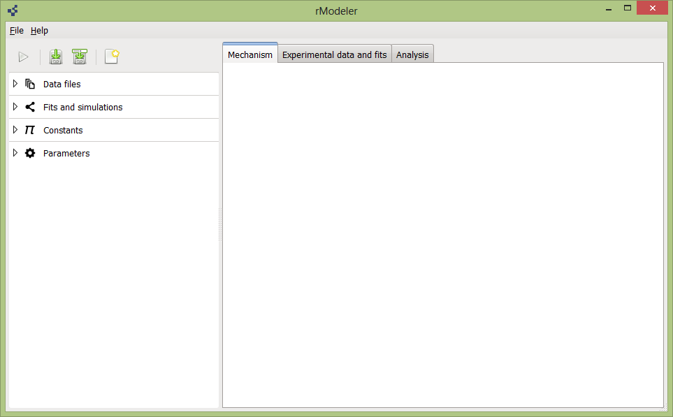
rModeler can be started by double clicking on rModeler icon in Desktop, or by looking up the application in Search Charm.
The rModeler application will look something like this on Windows 8:
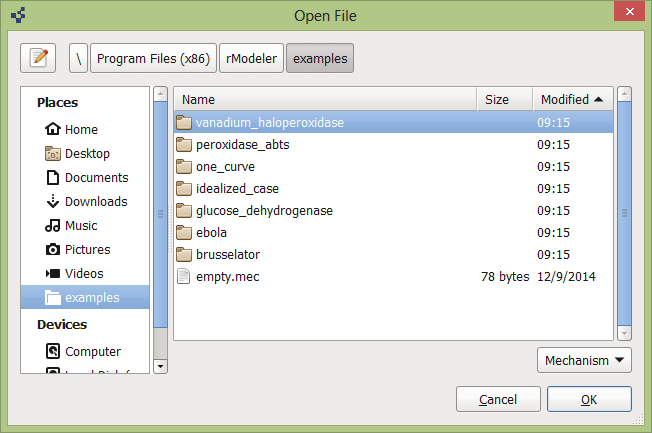
rModeler comes bundled with seven examples that differ in complexity and topic. Examples could be opened by selecting File menu on the top-left corner of the main window:

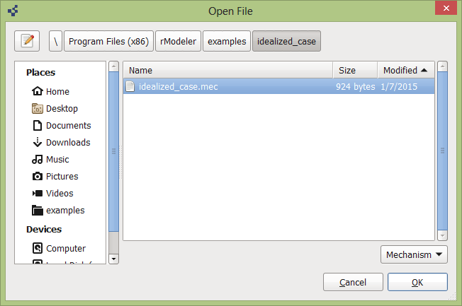
If you run the program in Windows 8, the examples directory can be quickly found on the left side of the Open File dialog, in Places sidebar. It is recommended to start with the idealised_case example. The same example is described in Introduction (1).
Project file is in idealized_case directory and has “.mec” extension. You will load it by selecting idealized_case.mec file and clicking “OK” button in dialog.
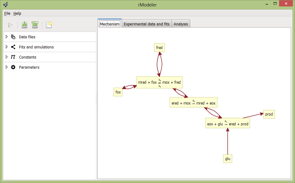
The opened project should look like this:
rModeler has 3 main tabs:
In the Mechanism tab you will see a graphical representation of the reaction scheme. The purpose of this graphical representation is to help visualize how participating reagents and reactions interact with each other.
If you would like to export the reaction scheme, simply right-click on the mechanism and the export pop-up will appear. You can export a mechanism as an *.eps, *.pdf, or a *.png file.
Naturally, the reaction scheme can be modified. If you would like to edit the reactions, simply double-click on the mechanism. A dialog that allows to add, remove or edit reactions will appear:

In Response equation field you should write a linear equation that describes how concentrations are converted into a measured quantity. For example, the molar absorptivity of potassium ferricyanide at \(420\ nm\) is \(1000\ M^{-1}cm^{-1}\), the optical path in the experiment is \(1 cm\). If your experiment only measures the change of ferricyanide absorbency in time, then your response equation will be \(1000*fox\) (here, we name ferricyanide as fox).
You can expand a reaction by clicking the small triangles on the left side of the dialog. A reaction is edited by changing the reaction equation (reactions can be in any order), defining plausible upper and lower logarithmic limits for the rate constants, (re)naming constants, or you can simply write out the actual numeric value for a rate constant in forward and backward fields. Symbolic values are expected to be optimized. Minimum and maximum are logarithmic values. Or you can simply delete reaction with cross button on reactions field right. Or even simpler – clicking New reaction to add new.

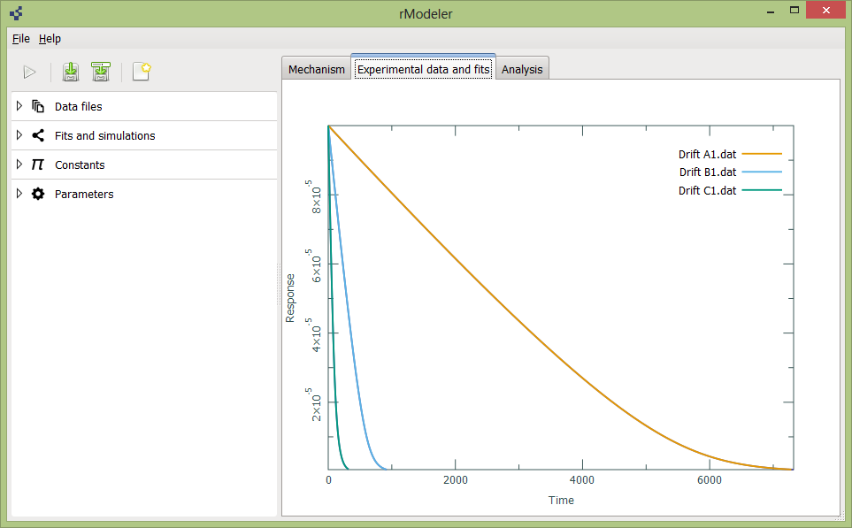
In Experimental data and fits tab are ploted all you data and simulations:
To add or delete data files, you should to expand data files tab on left:
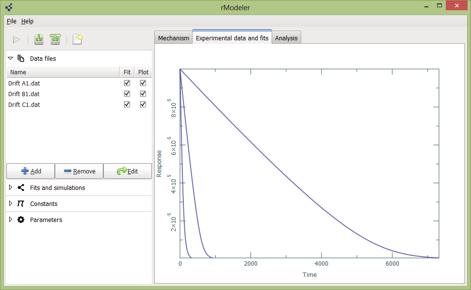
Using button Add you can browse and select your data files from your directories. Remove button removes them from project. Edit button call initial conditions dialog:

In which you should to provide all necessary initial concentrations for each experiment. Reagent species comes from mechanism. These initial conditions are used for numerical integration of reagents concentrations over time in your reaction scheme. When you fill up mechanism tab with reaction scheme, add initial conditions, fitting procedure could be started with Play button in the top left corner of rModeler window.
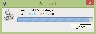
When fitting starts, you wil encounter two dialogs. Grid search, which indicates, how much you are expected to wait to perform grid search:
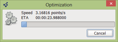
And Optimization, which show how much is left to wait:
When fitting procedure is completed, You will see legend and fits appeared in Experimental data and fits tab. You can expand Fits and simulations tab and here add new simulations with button Add, or remove simulations and fits with button Remove, or fill up initial conditions for new simulations with selecting simulation and clicking Edit button.
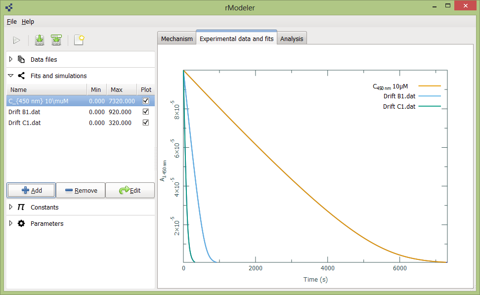
Also you can customize legend by simple edit of simulation name in Fits and simulations tab. Customization supports LaTex. Hitting “Tab” on your keyboar instantly updates legend in plot. Axes of plot also could be changed by cliking on axis title:
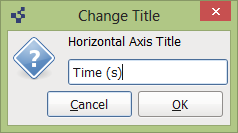
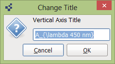
It supports LaTex too.
In Constants tab, you will see scroll bars, which can be slided and interactively changed values of rate constants. This is useful to play with them and inspect how much you simulation or fitting results are sensitive to rate constant change:

Rate constants could be changed exactly by clicking on constant name in constants tab.
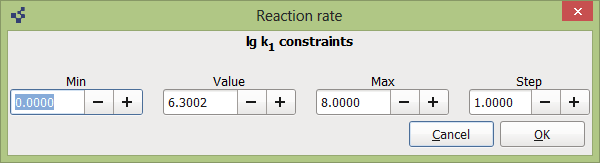
Here you can fix some simulation value, change Min, Max, Step values, which are used to determine rate constants grid.
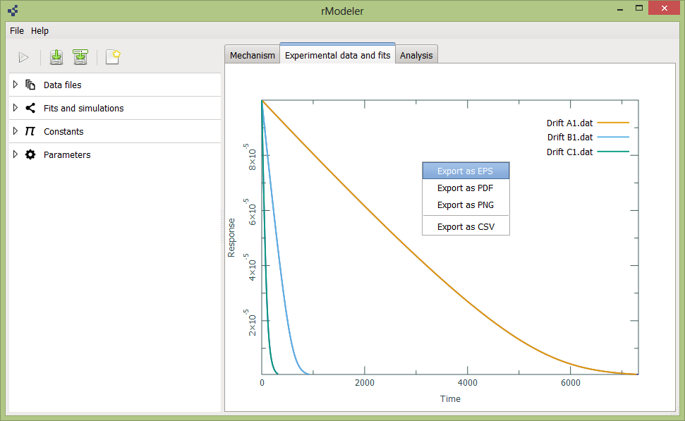
Numerical values of simulations and fits, plots for puplications could be exported with right mouse click:
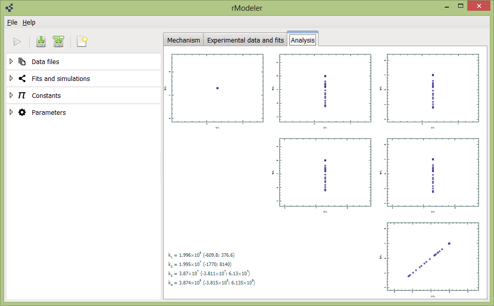
Analysis tab shows optimized rate constants values and their relation to each other. If you see linear relation between rate constants in same reaction, this is good reason to expect here equilibrium – then absolute rate constant doesnt matter, matters only ther ratio (in logarithmical scale – linear relation). This case is seen in last cross-plot. When you find constants relation as simple point in plot, this case indicate reasonably determinted rate constants. Variuos hyperbolic ralations are associated to consecutive or parallel reactions.
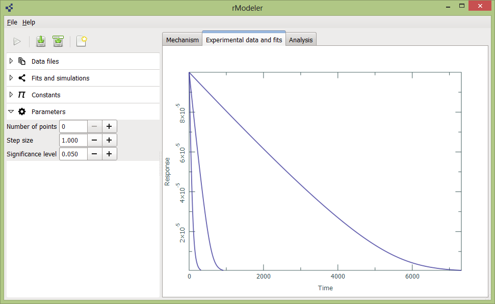
Parameters are closely associated to statistical analysis – here you could select Significance level, which is used to calculate your rate constant confidence intervals. Number of points determines, how much points after grid search should be selected for optimization (rule of thumb – \(3^{number\ of\ rate\ constants}\). Step size controls grid search coarseness (few rate constants – small step size, many rate constants – bigger step size, all depends how fast are your hardware).
1 Laurynenas, Audrius, and Kulys, Juozas. “An exhaustive search approach for chemical kinetics experimental data fitting, rate constants optimization and confidence interval estimation.” http://www.mii.vu.lt/na/issues/NA_2001/NA20110.pdf